Central Limit Theorem with Minitab
What is Central Limit Theorem?
The Central Limit Theorem is one of the fundamental theorems of probability theory. It states a condition under which the mean of a large number of independent and identically-distributed random variables, each of which has a finite mean and variance, would be approximately normally distributed. Let us assume Y1, Y2 . . . Yn is a sequence of n i.i.d. random variables, each of which has finite mean μ and variance σ2, where σ2 > 0. When n increases, the sample average of the n random variables is approximately normally distributed, with the mean equal to μ and variance equal to σ2/n, regardless of the common distribution Yi follows where i = 1, 2 . . . n.
Independent and Identically Distributed
A sequence of random variables is independent and identically distributed (i.i.d.) if each random variable is independent of others and has the same probability distribution as others. It is one of the basic assumptions in Central Limit Theorem. Consider the law of large numbers (LLN)—It is a theorem that describes the result of performing the same experiment a large number of times. According to the LLN, the average of the results obtained from a large number of trials should be close to the expected value, and will tend to become closer as more trials are performed. The following example will explain this further.
Central Limit Theorem Example
Let us assume we have 10 fair die at hand. Each time we roll all 10 die together we record the average of the 10 die. We repeat rolling the die 50 times until we will have 50 data points. Upon doing so, we will discover that the probability distribution of the sample average approximates the normal distribution even though a single roll of a fair die follows a discrete uniform distribution. Knowing that each die has six possible values (1, 2, 3, 4, 5, 6), when we record the average of the 10 dice over time, we would expect the number to start approximating 3.5 (the average of all possible values). The more rolls we perform, the closer the distribution would be to
Confidence Interval
The confidence interval is an interval where the true population parameter would fall within a certain confidence level. A 95% confidence interval, the most commonly used confidence level, indicates that the population parameter would fall in that region 95% of the time or we are 95% confident that the population parameter would fall in that region. The confidence interval is used to describe the reliability of a statistical estimate of a population parameter.
The width of a confidence interval depends on the:
- Confidence level—The higher the confidence level, the wider the confidence interval
- Sample size—The smaller the sample size, the wider the confidence interval
- Variability in the data—The more variability, the wider the confidence interval
Minitab: Calculate the Confidence Interval of the Mean
Data File: “Central Limit Theorem” tab in “Sample Data.xlsx”
- Click Stat → Basic Statistics → Graphical Summary.
- A new window named “Graphical Summary” pops up.
- Select “Cycle Time(Minutes)” as the variable.
- The confidence level is 0.95 by default.

- Click “OK.”
- A new window named “Summary for Cycle Time(Minutes)” pops up.

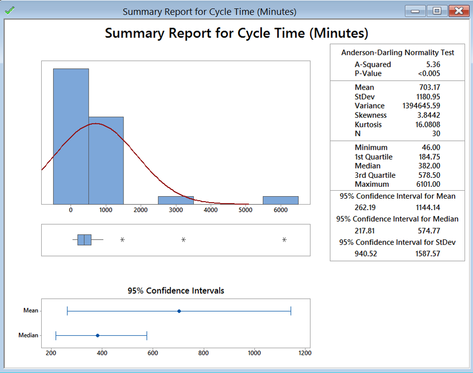
The 95% confidence interval of the mean is shown in the newly-generated “Summary for Cycle Time (Minutes).” The confidence level is 95% by default. In order to see the confidence interval of “Cycle Time (Minutes)” at other confidence level, we need to enter the confidence level of our interest in the window “Graphical Summary” and click “OK.”
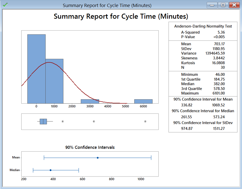
The following example shows how to generate 90% confidence interval of the mean.
 Model summary: Here the example shows what selections to make in Minitab to get the confidence intervals around the mean and standard deviation. While Minitab has the default confidence interval at 95%, you can see that other confidence levels can be selected as well.

